|
Telecons:
2021 July 09, 2021 July 02, 2021 June 25, 2021 June 18, 2021 June 11, 2021 June 4, 2021 May 28, 2021 May 21, 2021 May 14, 2021 (No meeting ISM2021 workshop) May 07, 2021 April 30, 2021 April 23, 2021 (ALMA deadline - no meeting) April 16, 2021 April 09, 2021 April 02, 2021 (Easter no meeting) March 26 2021 (ALMA-IMF Workshop telcon) March 19,2021 March 12, 2021 March 05,2021 February 26 2021 February 19 2021 February 12 2021 February 05 2021 January 29 2021 January 22 2021 January 15, 2021 January 8, 2021 2020 December 18, 2020 December 11, 2020 December 04, 2020 November 27, 2020 November 20, 2020 June 19, 2020 June 5, 2020 Feb 14 2020 Feb 7 2020 Jan 24 2020 January 10, 2020 ... 2019 October 18, 2019 October 11, 2019 October 4, 2019 September 2019 August 2019 July 2019 March 13, 2019 March 6, 2019
0 Comments
Time: Jul 3, 2019 09:00 AM Mountain Time (US and Canada) 1500 UTC https://ufl.zoom.us/j/236013059 Attendees: Adam Ginsburg, Fumitaka Nakamura, Brian Svoboda, Timea Csengeri, Roberto Galván, Sylvain Bontemps, Hongli Liu, Fredrique Motte, Yohan Pouteau, Fabien Louvet, Fernando Olguin, Amelia Stutz Agenda: https://github.com/ALMA-IMF/reduction/wiki/Reduction-Telecon-July-2019
5. If time allows, walk through self calibration instructions 6. Discussion of imaging issues related to specific images. Minutes: To be added during telecon Questions:
TODO:
Overview: Our goal is to have at least first-pass joint 12m imaging (both 12m configurations) for each of B3 and B6 by mid-August. We need to have the exact reduction script/process required to produce these files also. These do not have to be final products, but they must be images that we can discuss and use to make further decisions. Please fill out information about which field you are working on in the "Continuum Imaging result" tab of this table: https://docs.google.com/spreadsheets/d/1xM8AfiMpe8SVifqzl0lzjD10CEB2OlLIw_Kw5R1sxAM/edit#gid=1857654559 If you have FITS image files of the continuum already in hand, please share them with me and I will collect them in a single location for further inspection by the team or a subset of the team. Notes added before telecon: Add your region-specific notes below. Bold the heading so they show up in the “Outline” view to the left. Mosaic PSF * PB weighting: From Dirk’s reply to the helpdesk ticket (July 2, 2019): “OK, I talked to the imaging development people yesterday again. The fix is not going to be in 5.6 but probably in the version after that (5.7). However, they assured me that this is only affecting the case nterms>=2 for mosaics and even there the Stokes I flux is OK. Just the minor cycle alpha (spectral index) calculation is affected. There is a known workaround: Use the PSF made from gridder='standard' with the joint mosaic. So, run niter=0 with gridder='mosaic'. Then run niter=0 with gridder='standard'. Then copy over the imagename.psf to the names for the imaging run for gridder='mosaic' and restart the mosaic run with calcpsf=False. So, I'll regard this ticket as resolved now. I am told by the CASA people that there is nothing broken which could affect standard ALMA data analysis. “ Adam’s commentary: I don’t believe this affects the majority of our data sets significantly or perhaps at all, since our mosaics are symmetric. This issue means that, when a model component is added at a particular position in the mosaic, there will be no flux removed on a minor cycle from points >0.5x(mosaic width) from the image. However, the mosaic gridder already strictly enforces that each pointing has a pblimit=0.05, so this problem should have no perceivable effect on our imaging. For long linear mosaics, particularly L-shaped ones, it could be a problem. Adam’s notes on W51: Self-calibration has been successful. Clean with higher robust values (recovering more extended emission) has also worked reasonably well. A full analysis of the self-calibration is available: https://github.com/ALMA-IMF/notebooks/blob/master/W51E_B3_selfcal.ipynb https://github.com/ALMA-IMF/notebooks/blob/master/W51-E_B6_Selfcal.ipynb (if these don’t load, try pasting the URLs in http://nbviewer.jupyter.org) Notably, the B3 RMS dropped from ~0.31 mJy/beam (light cleaning, no self-cal) to ~0.08 mJy/beam (deep cleaning, self-calibrated). The total dynamic range went from ~850 to ~5400. pk/mad= 870.7, pk=0.266 Jy / beam, total=176.968 Jy / beam, mad=0.30520 mJy / beam, beam=0.29x0.26 pk/mad=2761.8, pk=0.409 Jy / beam, total=176.580 Jy / beam, mad=0.14800 mJy / beam, beam=0.29x0.26 pk/mad=3527.9, pk=0.410 Jy / beam, total=283.565 Jy / beam, mad=0.11623 mJy / beam, beam=0.29x0.26 pk/mad=4218.7, pk=0.410 Jy / beam, total=398.153 Jy / beam, mad=0.09730 mJy / beam, beam=0.29x0.26 pk/mad=4346.9, pk=0.410 Jy / beam, total=408.235 Jy / beam, mad=0.09442 mJy / beam, beam=0.29x0.26 pk/mad=4685.6, pk=0.410 Jy / beam, total=448.358 Jy / beam, mad=0.08757 mJy / beam, beam=0.29x0.26 pk/mad=5412.0, pk=0.409 Jy / beam, total=450.818 Jy / beam, mad=0.07561 mJy / beam, beam=0.29x0.26 In band 6, the results are similar but less extreme: peak/mad= 904.2, peak=0.272 Jy / beam, rms=0.00069 Jy / beam, mad=0.00030 Jy / beam, peak/mad=1735.1, peak=0.449 Jy / beam, rms=0.00061 Jy / beam, mad=0.00026 Jy / beam, peak/mad=1897.5, peak=0.474 Jy / beam, rms=0.00048 Jy / beam, mad=0.00025 Jy / beam, peak/mad=1901.7, peak=0.473 Jy / beam, rms=0.00048 Jy / beam, mad=0.00025 Jy / beam, peak/mad=1904.9, peak=0.473 Jy / beam, rms=0.00048 Jy / beam, mad=0.00025 Jy / beam, peak/mad=1927.4, peak=0.474 Jy / beam, rms=0.00042 Jy / beam, mad=0.00025 Jy / beam, peak/mad=2390.9, peak=0.475 Jy / beam, rms=0.00026 Jy / beam, mad=0.00020 Jy / beam, These images show the ALMA data (left) and VLA data (right) and their difference modulo a scaling factor (center) to highlight the dust emission. The 3 mm data have been self-calibrated with 5 iterations of phase-only selfcal and 2 of amplitude selfcal on the robust 0 data. The robust 2 images involved additional “custom” cleaning. 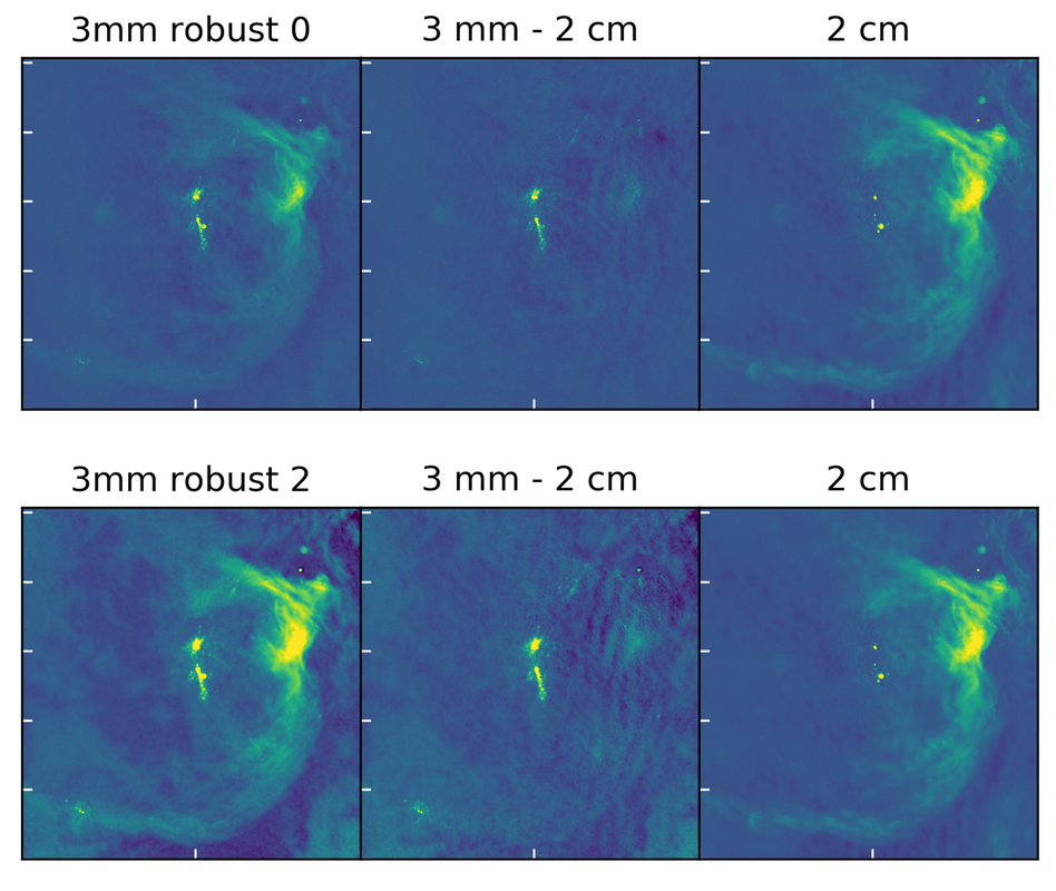 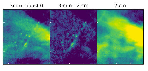 Part of results from Hongli/Amelia (Two parts in total: the first part is obtained without any self-calibration, the second with self-calibration): In a very short summary, our results were generated with the scripts in alma-imf repository. We have demonstrated them to be very practical, controllable, useful and resonable by applying to the source G353.41. In particular for the selfcalibration, to our experience, the phase calibration can improve the dynamical range of final images but not always significantly, depending on bands. For example, in the case of G353.41, band3 benefits a lot from self-calibration. However, the amplitude selfcalibration will get the flux decreased in both bands of G353.41, so we probably need to be very careful when doing the amplitude self-calibration. Below are examples of images of several parameters (i.e., flux, model, residual, and mask) for two types of combinations (i.e., 12m, and 12m+7m) at the robust parameter 0 (I also have done for other robust parameters -2 0.5 2. BTW, what robust parameter(s) will be used at last) without selfcal in both band 3. 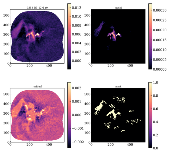 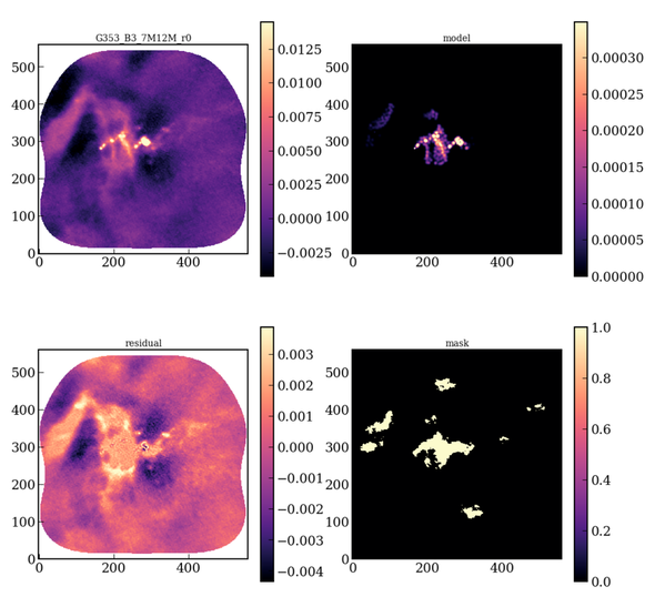 Below are examples of images of several parameters (i.e., flux, model, residual, and mask) for two types of combinations (i.e., 12m, and 12m+7m) at the robust parameter 0 without selfcal in both band 6. 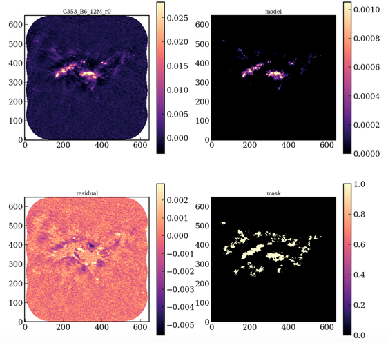 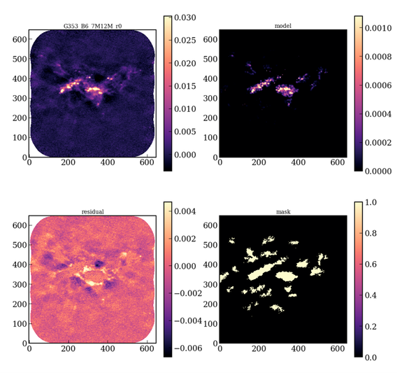 The same as above but with three-time iterations of phasecal for band 3 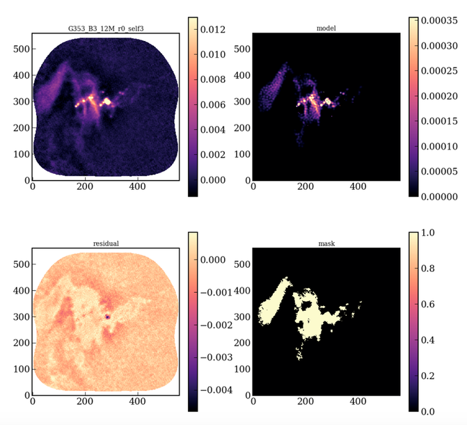 The same as above but with three-time iterations of phasecal for band 6 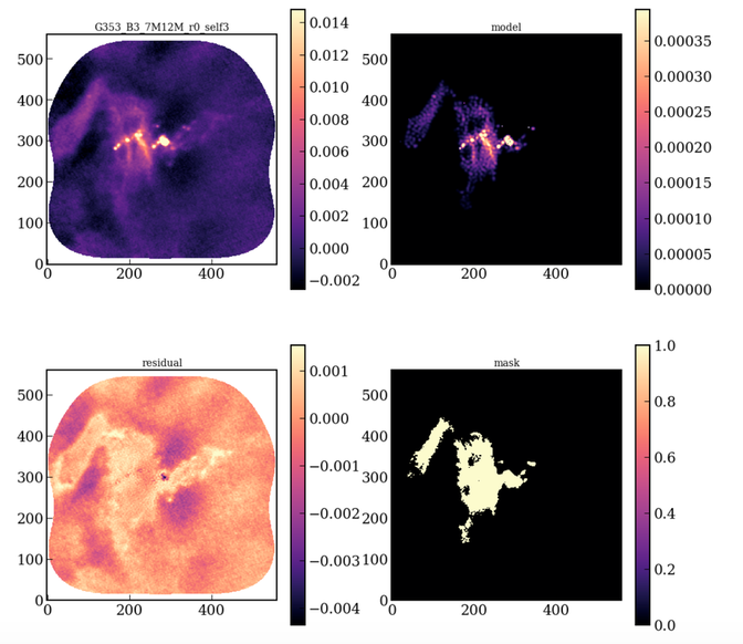 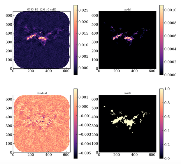 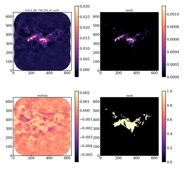 The list of several critical parameters (i.e., maximum flux, rms, dynamical range) for comparison of images between with and without selfcal. Note that we did six-times selfcalibration including four times on phase, and two times on amplitude. You will see below how the dynamical range and the maximum flux change with each calibration. First, let’s look at the results of Band3 for source G353.41 #without self-cal 'G353_B3_12M_r0': {'max': '0.19 Jy / beam', 'rms': '0.39 mJy / beam', 'drange': '471.70' #phase self-cal 'G353_B3_12M_r0_self1': {'max': '0.19 Jy / beam', 'rms': '0.32 mJy / beam', 'drange': '573.22', 'G353_B3_12M_r0_self2': {'max': '0.19 Jy / beam', 'rms': '0.27 mJy / beam', 'drange': '676.93', 'G353_B3_12M_r0_self3': {'max': '0.19 Jy / beam', 'rms': '0.27 mJy / beam', 'drange': '692.39', 'G353_B3_12M_r0_self4': {'max': '0.19 Jy / beam', 'rms': '0.27 mJy / beam', 'drange': '693.12', # amplitude self-cal comes from below 'G353_B3_12M_r0_self5': {'max': '0.19 Jy / beam', 'rms': '0.28 mJy / beam', 'drange': '656.17', 'G353_B3_12M_r0_self6': {'max': '0.18 Jy / beam', 'rms': '0.28 mJy / beam', 'drange': '662.36', Second, let’s look at the results of Band6 for source G353.41 #without self-cal 'G353_B6_12M_r0': {'max': '0.11 Jy / beam', 'rms': '0.65 mJy / beam', 'drange': '167.18', #phase self-cal 'G353_B6_12M_r0_self1': {'max': '0.10 Jy / beam', 'rms': '0.65 mJy / beam', 'drange': '158.66', ‘'G353_B6_12M_r0_self2': {'max': '0.10 Jy / beam', 'rms': '0.61 mJy / beam', 'drange': '170.10', 'G353_B6_12M_r0_self3': {'max': '0.10 Jy / beam', 'rms': '0.61 mJy / beam', 'drange': '171.05', 'G353_B6_12M_r0_self4': {'max': '0.10 Jy / beam', 'rms': '0.61 mJy / beam', 'drange': '171.10', # amplitude self-cal comes from below 'G353_B6_12M_r0_self5': {'max': '0.10 Jy / beam', 'rms': '0.62 mJy / beam', 'drange': '167.04', 'G353_B6_12M_r0_self6': {'max': '0.10 Jy / beam', 'rms': '0.60 mJy / beam', 'drange': '164.84', Imaging_parameters required in the scripts from the alma-imf repository are below for the source G353.41 # for dirty (the first run) imaging_parameters_nondefault = { #12M of band 3 'G353.41_B3_12M_robust0': {'threshold': '1.8mJy', # 4*RMS 'scales': [0,3,9], }, 'G353.41_B3_12M_robust0.5': {'threshold': '2.0mJy', # 4*RMS 'scales': [0,3,9], }, 'G353.41_B3_12M_robust-2': {'threshold': '1.8mJy', # 4*RMS 'scales': [0,3,9], }, 'G353.41_B3_12M_robust2': {'threshold': '3.3mJy', # 4*RMS 'scales': [0,3,9], }, #7M12M of band 3 'G353.41_B3_7M12M_robust0': {'threshold': '4mJy', # 4*RMS 'scales': [0,3,9], }, 'G353.41_B3_7M12M_robust0.5': {'threshold': '4.0mJy', # 4*RMS 'scales': [0,3,9], }, 'G353.41_B3_7M12M_robust-2': {'threshold': '4.4mJy', # 4*RMS 'scales': [0,3,9], }, 'G353.41_B3_7M12M_robust2': {'threshold': '4.8mJy', # 4*RMS 'scales': [0,3,9], }, #12M of band 6 'G353.41_B6_12M_robust0': {'threshold': '2.2mJy', # 4*RMS 'scales': [0,3,9], }, 'G353.41_B6_12M_robust0.5': {'threshold': '1.5mJy', # 4*RMS 'scales': [0,3,9], }, 'G353.41_B6_12M_robust-2': {'threshold': '2.9mJy', # 4*RMS 'scales': [0,3,9], }, 'G353.41_B6_12M_robust2': {'threshold': '1.6mJy', # 4*RMS 'scales': [0,3,9], }, #7M12M of band 6 'G353.41_B6_7M12M_robust0': {'threshold': '2.3mJy', # 4*RMS 'scales': [0,3,9], }, 'G353.41_B6_7M12M_robust0.5': {'threshold': '2.3mJy', # 4*RMS 'scales': [0,3,9], }, 'G353.41_B6_7M12M_robust-2': {'threshold': '3.12mJy', # 4*RMS 'scales': [0,3,9], }, 'G353.41_B6_7M12M_robust2': {'threshold': '3.3mJy', # 4*RMS 'scales': [0,3,9], } } # for selfcal1, selfcal2,self.... imaging_parameters_nondefault_self = { #12M of band 3 'G353.41_B3_12M_robust-2': {'threshold': '1.2mJy', # 4*RMS 'scales': [0,3,9], }, 'G353.41_B3_12M_robust0': {'threshold': '0.9mJy', # 4*RMS 'scales': [0,3,9], }, 'G353.41_B3_12M_robust0.5': {'threshold': '1.0mJy', # 4*RMS 'scales': [0,3,9], }, 'G353.41_B3_12M_robust2': {'threshold': '1.3mJy', # 4*RMS 'scales': [0,3,9], }, #7M12M of band 3 'G353.41_B3_7M12M_robust-2': {'threshold': '1.8mJy', # 4*RMS 'scales': [0,3,9], }, 'G353.41_B3_7M12M_robust0': {'threshold': '1.6mJy', # 4*RMS 'scales': [0,3,9], }, 'G353.41_B3_7M12M_robust0.5': {'threshold': '1.6mJy', # 4*RMS 'scales': [0,3,9], }, 'G353.41_B3_7M12M_robust2': {'threshold': '2.1mJy', # 4*RMS 'scales': [0,3,9], }, #12M of band 6 'G353.41_B6_12M_robust-2': {'threshold': '2.9mJy', # 4*RMS 'scales': [0,3,9], }, 'G353.41_B6_12M_robust0': {'threshold': '2.1mJy', # 4*RMS 'scales': [0,3,9], }, 'G353.41_B6_12M_robust0.5': {'threshold': '1.5mJy', # 4*RMS 'scales': [0,3,9], }, 'G353.41_B6_12M_robust2': {'threshold': '1.6mJy', # 4*RMS 'scales': [0,3,9], }, #7M12M of band 6 'G353.41_B6_7M12M_robust-2': {'threshold': '3.0mJy', # 4*RMS 'scales': [0,3,9], }, 'G353.41_B6_7M12M_robust0': {'threshold': '2.2mJy', # 4*RMS 'scales': [0,3,9], }, 'G353.41_B6_7M12M_robust0.5': {'threshold': '1.7mJy', # 4*RMS 'scales': [0,3,9], }, 'G353.41_B6_7M12M_robust2': {'threshold': '2.0mJy', # 4*RMS 'scales': [0,3,9], }, } Roberto’s notes on G333.60 B3: Adam visited Morelia during the spring and we set-up the imaging scripts to work for B3. The main result is that we have acceptable 12m-array (both configs), self-calibrated, robust 0 images. The continuum subtraction is for the “cleanest”, pipeline-defined continuum. Selfcal significantly improved the noise and S/N in the images. Three iterations of phase- and one iteration of ap-selfcal were applied. I did some tests to try to automatize the cleaning windows using auto-multithresh without satisfactory results. In the end, self-cal was done through a scripted way but defining the cleaning masks by eye in a previous interactive cleaning, and saving them for posterior use. Details below. - Step 1: run continuum_imaging_both.py with interactive=True. I edited it to do only robust = 0, exclude 7m, and do only ‘cleanest’ continuum, since the ‘best sensitivity’ continuum option takes much longer to run. Since the purpose of this cleaning run was to define self-cal masks, I first cleaned shallowly the brightest central emission, and successively cleaned more exterior, fainter emission. The four ‘masks’ can be found in the link. I saved them in CASA in crtf format, but I think the scripts accept other formats, such as ds9 or a true mask image. Note that each successive mask includes the area in the previous one. https://www.dropbox.com/s/jh0j1et9owgb7zf/selfcal_masks_G333B3.tar?dl=0 - Step 2: run continuum_imaging_selfcal.py, editing imaging_parameters.py to include the name of the cleaning masks and the selfcal parameters for each iteration. The scripts that I used can be found in the link. Note that imaging_parameters file is only for G333 (should rename without ‘G333’ for it to run), so I haven’t done this in the framework of including all the params for all targets in a single imaging_parameters file. https://www.dropbox.com/s/vruh2x0rosrxjr8/selfcal_scripts_G333B3.tar?dl=0 Results: Improvement over the selfcal iterations can be seen in the following animated gif: 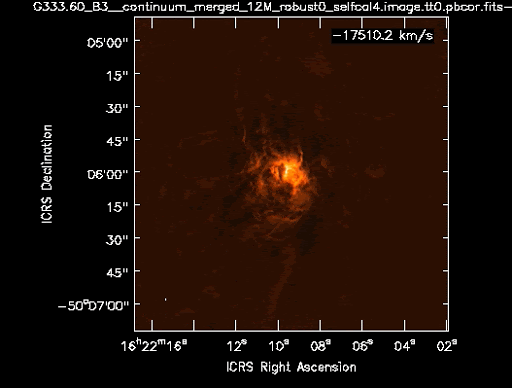 The non-pbcor fits images can be found here:
https://www.dropbox.com/s/iom9d2mhit2l834/selfcal_fits_G333B3.tar?dl=0 Image rms noise Peak S/N (mJy/b) (mJy/b) No-selfcal 0.252 189 750 Selfcal p1 0.250 198 792 Selfcal p2 0.153 200 1307 Selfcal p3 0.108 203 1880 Selfcal ap 0.079 194 2456 The final ap selfcal has 4% less peak flux than the previous phase-only selfcal, but looks better and has better S/N. - Step 3: do a final clean on the final selfcal ms. interactive=True should be better, but clean masks will be saved to be able to run it in a script. Question for telecon: do this within continuum_imaging_selfcal.py? Another script? - Other tests: Roberto’s tests of automultithresh: 1) Played a bit with parameters of automultithresh. My conclusion is that one cannot get to something as good as the masks that I defined by eye. Below a comparison of an automatic mask (white pixels) with one of the by-eye masks (regions) used in the selfcal Minutes for ALMA-IMF telecon, March 13, 2019 Agenda: https://github.com/ALMA-IMF/reduction/wiki/ALMA-IMF-Data-Reduction-Telecon,-March-13,-2019 http://desktop.visio.renater.fr/scopia?ID=722288***2252&autojoin Attendees: Adam Ginsburg, Roberto Galván,Hongli Liu, Patricio Sanhueza, Nichol Cunningham, Jonathan Braine, Fernando Olguin, Brian Svoboda, Thomas Nony Imaging results:

 B6: only 12M. sidelobethreshold=2, noisethreshold=4.25 (from casaguide). negativethreshold=1000 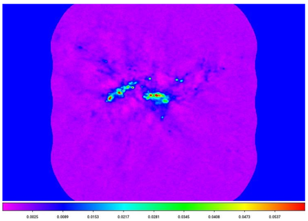 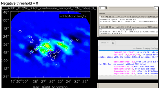 Discussion of imaging parameter saving:
https://github.com/ALMA-IMF/reduction/pull/10/files Masking and thresholding discussion:
This is what I used for line cleaning, some kind of auto-masking tclean. It worked quite well in IRDCs. http://adsabs.harvard.edu/abs/2018ApJ...861...14C (see also https://home.strw.leidenuniv.nl/~ycontreras/yclean.html -> https://home.strw.leidenuniv.nl/~ycontreras/yclean.py ) Agenda: https://github.com/ALMA-IMF/reduction/wiki/ALMA-IMF-Data-Reduction-Telecon,-March-6,-2019 Minutes: Participating: Adam Ginsburg, Frederique Motte, Patricio Sanhueza, Brian Svoboda, Ana Lopez, Jordan Molet, Thomas Nony, Sylvain Bontemps, Fernando Olguin, Roberto, Hongli Liu
W51 examples from Adam, lines excluded: Left: Before: no selfcal ; Right: after 1 iter selfcal G327 from Patricio B6 lines excluded, no selfcal (selfcal is needed): 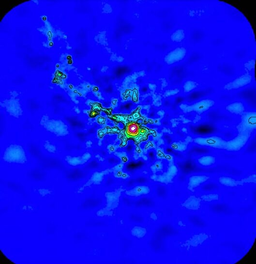 |
Archives
July 2021
Categories
|


 RSS Feed